Citi Bike Demand Forecaster:Live 24-Hour Prediction Pipeline
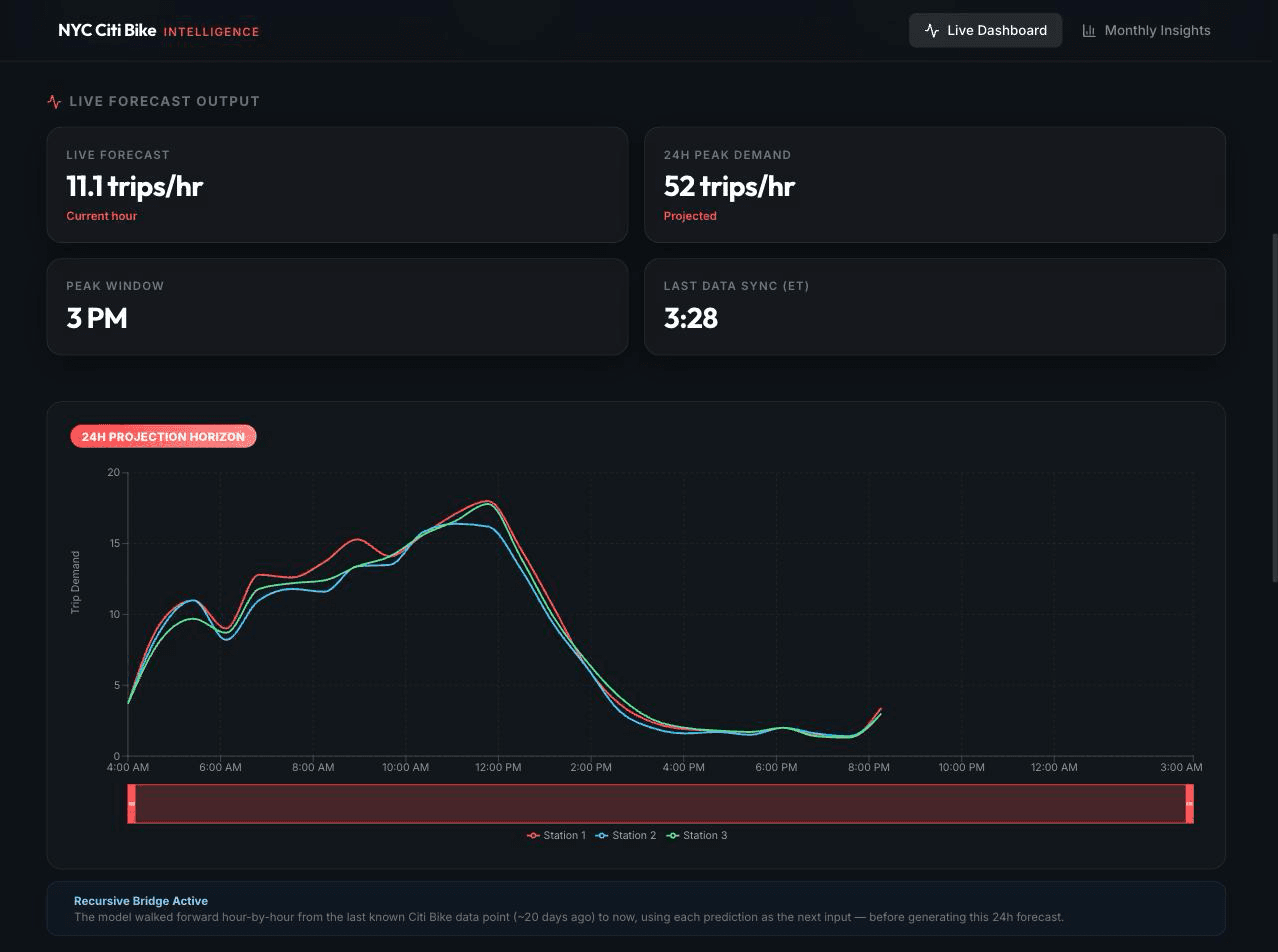
Live NYC Citi Bike demand forecaster serving a 28-hour recursive-multistep LightGBM forecast for the 3 busiest stations. A two-phase Recursive Bridge walks the ~20-day public-data lag forward to the present, so the model can predict tomorrow from data that stops three weeks ago.
Core Impact
“Turns a dataset published ~20 days late into a live 28-hour forecast at MAE 2.94 trips/hour, fully automated through 3 scheduled GitHub Actions workflows and served at $0 backend cost.”
2.94
MAE, trips per hour
28 hr
Recursive forecast horizon
$0
Backend cost, S3 Parquet direct
The Problem
Citi Bike publishes its trip data about 20 days behind, which quietly makes the public dataset useless for real-time prediction. Any model trained on it is forecasting from a picture of three weeks ago. I wanted an operator-facing forecast of the next 28 hours anyway, which meant solving the lag itself before the forecasting even starts.
The Approach
Why a two-phase Recursive Bridge
Phase one walks the model forward hour by hour from the last real observation to now, feeding its own predictions back in as lag features. Phase two forecasts the actual 28 hours ahead from that bridged present. Without the bridge there is simply no way to predict tomorrow from data that stops three weeks ago.
Why LightGBM instead of a neural model
The signal here is lag features and station identity, which gradient boosting handles directly, including categoricals with no encoding layer. It trains in seconds inside a GitHub Actions runner and lands at MAE 2.94 trips/hour, so a heavier architecture would cost more and buy nothing.
Why one model for three stations
Each station gets 28 lag features plus its own categorical ID, so a single model learns the shared temporal shape while still separating station-specific demand. Three separate models would triple the retrain and registry surface for no accuracy gain.
Why three separate Actions workflows
Feature ETL and retraining run monthly, inference runs hourly. Splitting them means a failed retrain never blocks the hourly forecast, and each has its own schedule and its own failure surface instead of one fragile cron doing everything.
Why S3 Parquet with no API
Predictions are written to S3 as Parquet and the Next.js frontend reads them directly. Nothing stays running between forecasts, so operating cost is roughly zero, and the model registry in Hopsworks with MLflow lineage on DagsHub still gives full reproducibility.
Technical Deep Dive
Built a live demand forecaster predicting NYC Citi Bike usage on a 28-hour recursive horizon, driven by 3 independent GitHub Actions workflows (monthly feature ETL, monthly retrain, hourly inference) with zero manual intervention.
Engineered a two-phase Recursive Bridge that closes the ~20-day public data lag, feeding predictions back as features to walk from the last real observation to the present before forecasting forward; achieved MAE 2.94 trips/hour on LightGBM.
Engineered per-station 28-lag features with native LightGBM categorical encoding across the 3 busiest stations, so a single model serves all of them while preserving station-specific demand patterns.
Built a Champion/Challenger registry with minimum-MAE promotion from the Hopsworks Model Registry and full lineage in MLflow on DagsHub; predictions archived to AWS S3 as Parquet.
Served the whole thing at $0 backend cost: the Next.js frontend parses S3 Parquet directly with PyArrow-written files, so there is no always-on API to pay for.
Systems Analysis Concluded